https://www.youtube.com/watch?v=28QbrkRkHlo&t=5526s
게시글의 내용의 대부분은 위 영상을 참고하며 작성했다.
질 좋은 강의를 무료로 공개하셔서 공부하는데 크게 도움이 될 것이다.
딥러닝을 학습함에 있어서 필요한 요소로는 크게 네가지로 분류할 수 있다.
- 모델을 구성하는 layer
- 입력데이터와 출력값
- 학습시에 사용할 loss function
- 학습 진행방식을 결정하는 optimizer
딥러닝의 기본구조에 대한 개념이 있다고 가정하고 keras와 tensorflow를 사용하여 모델을 쌓는 방법에 대해 알아보려한다.

Layer
인풋레이어와 아웃풋 레이어를 제외하고 사이의 층, 위 그림의 노란색 노드들을 layer이라고 할 수 있으며 신경망의 핵심데이터 구조이다.
하나이상의 텐서를 입력받아 하나이상의 텐서를 출력한다.
역전파 방법과 체인룰을 이용하여 가중치를 업데이트하며 계산하는 층이라고 할 수 있다.
텐서플로와 케라스에서 주로 사용하는 레이어는 크게
- Dense
- Activation
- Flatten
- Input
으로 나뉜다 물론 cnn의 conv도 레이어라고 할 수 있지만 추후에 다루도록하자
from tensorflow.keras.layers import Dense, Activation, Flatten, Input
1. Dense
- 완전연결계층 (fully-connected layer) 으로 딥러닝 학습의 핵심 구조라고 할 수 있다.
- 노드의 수와 activation을 지정해야한다.
- name을 통하여 레이어간의 구분이 가능하다.
- 가중치 초기화
* 신경망의 성능에 큰 영향을 주는 요소
* 동일한 데이터로 학습시키더라도 가중치의 초기값에 따라서 성능차이가 날 수 있음.
* 보통 가중치의 초기값으로 0에 가까운 무작위 값을 사용
* keras에서는 기본적으로 glorot uniform, zero bias로 초기화함.
* kenel_initializer인자를 통해 다른 방법을 선택가능하다. (https://keras.io/api/layers/initializers/)
# 기본적인 사용 Dense(노드수, activation='활성화함수')
Dense(10, activation='softmax')

# Dense(노드수, activation='활성화함수', name='구분을위한(추후 summary 등이름설정'))
Dense(10, activation='relu', name='Dense Layer')

# Dense(노드수, activation='활성화함수', name='이름', kernel_initializer='가중치초기화 선택'))
Dense(10, kernel_initializer='he_normal', name='Dense Layer')
2. Activation
- Dense에서 정의할 수 있다
- 필요에 따라 별도 레이어를 만들 수 있지만 생략한다.
- https://keras.io/ko/activations/
dense = Dense(10, activation='relu', name='Dense Layer')
Activation(dense)
3. Flatten
- 배치크기 또는 데이터크기를 제와하고 데이터를 1차원으로 쭉펼치는 작업이다.
- ex) (128, 3, 2, 2) -> (128,12)
Flatten(input_shape=(128,3,2,2))
4. Input
- 모델의 입력을 정의한다.
- shape, dtype등을 지정한다.
- summary 메소드에는 보이지 않는다.
Input(shape=(28,28), dtype=tf.float32)
Input(shape=(28,), dtype=tf.int32)
Model
위에서 언급한 layer들을 쌓아 하나의 모델을 구성한다.
tf에서 제공하는 모델을 쌓는 방법은 세가지가있다.
- Sequential()
- 함수형 API
- 서브클래싱
모델구성
각 방법으로 모델을 쌓는 방법을 알아보자
1. Sequential()
- 모델이 순차적인 구조만을 가질 때에 사용한다.
- 가장 간단한 방법이라고 할 수 있으며 객체 생성이후 추가하는 방법, 한번에 리스트에 쌓는 방법이 있다
- 다중 입출력이 존재하는 등의 복잡한 모델을 구성할 수 없다.
* 객체에 쌓기
from tensorflow.keras.layers import Dense, Flatten, Activation, Input
from tensorflow.keras.models import Sequential, Model
from tensorflow.keras.utils import plot_model
model = Sequential()
model.add(Input(shape=(28, 28)))
model.add(Flatten(input_shape=[28,28]))
model.add(Dense(300, activation='relu'))
model.add(Dense(100, activation='relu'))
model.add(Dense(10, activation='softmax'))
model.summary()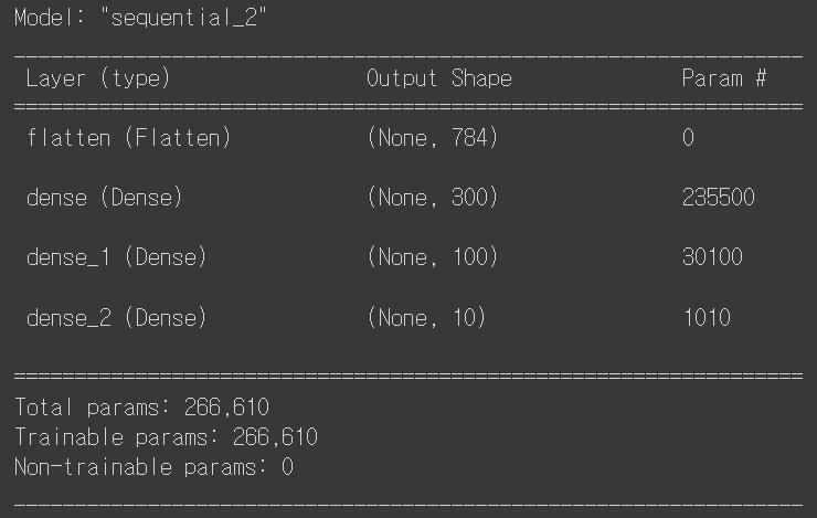
1) 먼저 28,28짜리의 데이터를 입력받으면
2) 28*28 = 784, 로 쭉펼친뒤에
3) 노드수가 300개인 층을 통과시킨다 우측 params를 보게 되면 235500을 볼 수 있는데
784(전 노드의 수)*300 (각 가중치) + 300(각 편향)을 의미한다.
4) 노드수가 100개인 층을 통과시킨다
300(전 노드의 수)*100 (각 가중치) + 100(각 편향)
5) 최종적으로 10개의 값을 출력한다.
total params 는 우측 params를 모두 더한 값이 나온다. 모델에서 찾아야하는 값이 266610이라는 뜻이다.
plot_model(model)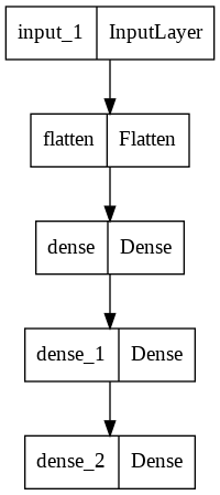
먼저 모델을 쌓을 틀을 만들고 그 위에 하나 하나 층을 쌓는 방법이다.
plot_model 을 이용하면 모델의 구조를 이미지로 확인가능하다.
* 리스트에 쌓기
model = Sequential([Input(shape=(28, 28), name='input'),
                    Flatten(input_shape=[28,28], name='Flatten'),
                    Dense(300, activation='relu', name='Dense1'),
                    Dense(100, activation='relu', name='Dense2'),
                    Dense(10, activation='softmax', name='Output')])

model.summary()
위와 같은 모델을 리스트를 이용한 방법으로 구성한 것이다.
2. 함수형 API
- 가장 권장되는 방법
- 모델을 복잡하고 유연하게 구성가능하다.
- 다중입출력을 다룰 수 있다.
inputs = Input(shape=(28,28,1))
x = Flatten(input_shape=(28,28,1))(inputs)
x = Dense(300, activation='relu')(x)
x = Dense(100, activation='relu')(x)
x = Dense(10, activation='softmax')(x)

model = Model(inputs=inputs, outputs=x)
model.summary()
위의 모델을 함수형 api를 이용하여 구현하는 코드이다.
이번에는 다중입출력인 경우를 보자
from tensorflow.keras.layers import Concatenate

input_layer = Input(shape=(28,28))
hidden = Dense(300, activation='relu')(input_layer)
hidden1 = Dense(30, activation='relu')(hidden)
concat = Concatenate()([input_layer, hidden1])
output = Dense(1)(concat)

model = Model(inputs=[input_layer], outputs=[output])
model.summary()

plot_model(model)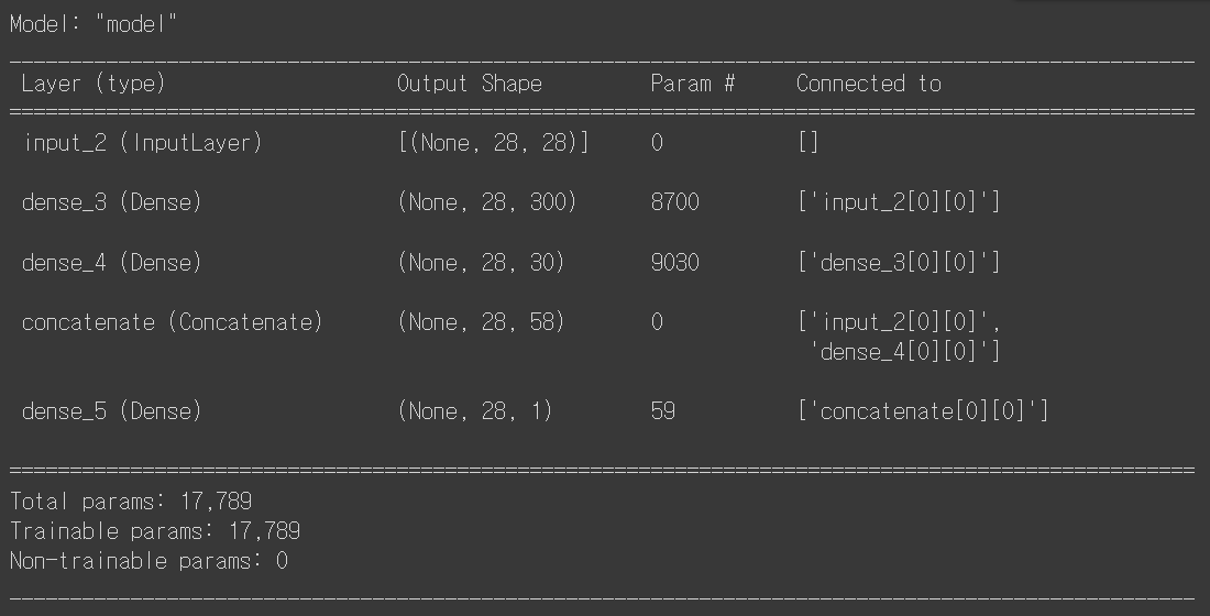
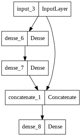
함수형을 활용하면 이렇게 여러가지의 경우를 구현 가능하다. 층이 깊어지면 이전의 가중치가 소실되는 경우가 있는데 이를 보완하기 위해 위같은 방법을 이용한다고 한다.
input_1 = Input(shape=(10,10), name='input_1')
input_2 = Input(shape=(10,28), name='input_2')

hidden_1 = Dense(100, activation='relu', name='hidden1')(input_2)
hidden_2 = Dense(10, activation='relu', name='hidden2')(hidden_1)

concat = Concatenate()([input_1,hidden_2])
output = Dense(1, activation='sigmoid', name='output')(concat)
sub_out = Dense(1, name='sum_output')(hidden_2)

model = Model(inputs=[input_1, input_2], outputs=[output, sub_out])
model.summary()
plot_model(model)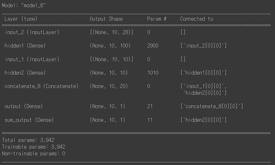
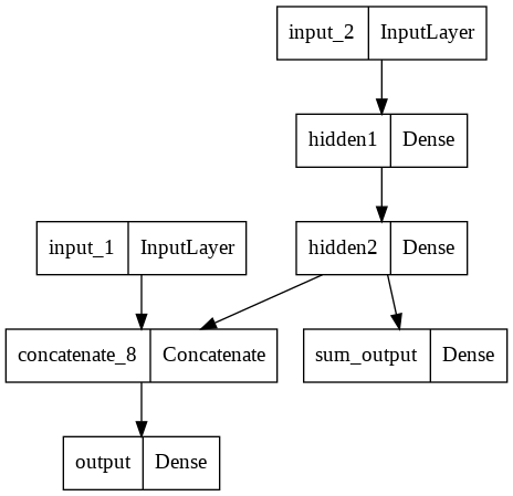
이렇게 복잡한 수준의 모델도 구현 가능하다.
3. 서브클래싱
- 커스터마이징에 최적화된 방법이다.
- model 클래스를 상속받아 포함된 기능을 사용할 수 있다.
* fit, evaluate, predict
* load, save
- 주로 call 메소드 안에서 원하는 계산이 가능하다
- 권장되는 방법은 아니지만 어떤 모델의 구현 코드를 보고 해석이 가능해야한다.
class mymodel(Model):
  def __init__(self, unit=30, activation='relu', **kwargs):
    super(mymodel, self).__init__(**kwargs)
    self.dense_layer1 = Dense(300, activation=activation)
    self.dense_layer2 = Dense(100, activation=activation)
    self.dense_layer3 = Dense(units, activation=activation)
    self.output_layer = Dense(10, activation='softmax')

  def call(self, inputs):
    x = self.dense_layer1(inputs)
    x = self.dense_layer2(x)
    x = self.dense_layer3(x)
    x = self.output_layer(x)
    return x
모델 가중치확인
inputs = Input(shape=(28,28,1))
x = Flatten(input_shape=(28,28,1))(inputs)
x = Dense(300, activation='relu')(x)
x = Dense(100, activation='relu')(x)
x = Dense(10, activation='softmax')(x)

model = Model(inputs=inputs, outputs=x)
model.summary()model.layers[<keras.engine.input_layer.InputLayer at 0x7f911aa41090>,
<keras.layers.core.flatten.Flatten at 0x7f911aa41d90>,
<keras.layers.core.dense.Dense at 0x7f911a6af950>,
<keras.layers.core.dense.Dense at 0x7f911a6af590>,
<keras.layers.core.dense.Dense at 0x7f911aa53590>]layer메소드를 이용하면 각 층에 접근할 수 있는데.
hidden_2 = model.layers[2]
hidden_2.name'dense_27'리스트안에 인덱싱으로 각 레이어에 접근가능하다.
weights, biases = hidden_2.get_weights()
print(weights.shape)
print(biases.shape)

print(weights[:5])
print(biases[:5])
(784, 300)
(300,)
[[ 0.0649123 0.0568922 0.0244069 ... 0.0261239 -0.0731153 -0.0429611]
[-0.0251026 -0.0474078 -0.0255548 ... 0.0275116 -0.0723424 0.0565901]
[-0.0404508 0.004266 0.0089313 ... -0.0602168 0.0643739 0.0600661]
[-0.0161134 0.0169627 -0.0641473 ... -0.0534405 0.0665736 0.0594366]
[ 0.0240779 0.0698114 0.0545021 ... 0.014021 0.0201097 -0.0600637]]
[0. 0. 0. 0. 0.]각 레이어에 get_weights 메소드로 가중치를 확인 가능하다.
현재는 학습이 진행되지않았기때문에 각 initializer의 초기값상태이다.
다음에는 모델의 학습과 컴파일 부분을 게시하겠다.
'TF' 카테고리의 다른 글
| [TF] CNN 컨볼루션 신경망 (0) | 2022.04.13 |
|---|---|
| [TF] 딥러닝 학습기술 (0) | 2022.04.12 |
| [TF] 모델의 저장, callbacks (0) | 2022.04.11 |
| [TF] 모델 컴파일 및 학습 mnist (0) | 2022.04.11 |