https://www.youtube.com/watch?v=28QbrkRkHlo&t=5526s
대부분 위의 영상을 참고했다.
모델 컴파일 (compile)
- 학습시에 사용할 loss function
- 학습 진행방식을 결정하는 optimizer
- 모델을 모니터링할 지표를 설정하는 단계이다.
model.compile(loss='sparse_categorical_crossentropy',
              optimizer='sgd',
              metrics=['accuracy'])
모델을 정의하고 loss, optimizer를 설정한다.
1. 손실함수 (loss function)
- 학습이 진행되면서 얼마나 잘되고 있는지 확인할 지표
- 모델이 훈련되면서 최소화될 값
- 손실함수에 따라서 학습파라미터fmf whwjd
- 미분가능한 함수를 사용
- loss 설정 detail https://keras.io/api/losses/probabilistic_losses/#kldivergence-function
- 주요 손실함수
* 분류
categorical_crossentropy (원핫 인코딩되어있는 라벨데이터에 사용)
sparse_categorical_crossentropy (다중분류)
binary_crossentropy (이진분류)
* 회귀
mean_squared_error
mean_absolute_error ( mse에 비해서 좀 더 이상치에 강건함)
2. 옵티마이저 (optimizer)
- 손실함수를 기반으로 모델이 파라미터가 어떻게 업데이터 되어야하는지 결정한다,
- https://keras.io/ko/optimizers/
- 옵티마이저의 튜닝을 위해 따로 객체를 생성하여 컴파일 하기도한다.
*
from keras import optimizers

model = Sequential()
model.add(Dense(64, kernel_initializer='uniform', input_shape=(10,)))
model.add(Activation('softmax'))

sgd = optimizers.SGD(lr=0.01, decay=1e-6, momentum=0.9, nesterov=True)
model.compile(loss='mean_squared_error', optimizer=sgd)
위의 예와 같은방법으로
- 주요 옵티마이저
keras.optimizer.SGD(): 기본적인 확률적 경사 하강법
keras.optimizer.Adam(): 자주 사용되는 옵티마이저
3. metrics
- 모니터링하는 지표
- loss function 이랑 비슷하지만 metric은 모델을 학습하는데 사용되지 않는다는 점에서 다름.
- 커스텀 metric
*
import keras.backend as K

def mean_pred(y_true, y_pred):
    return K.mean(y_pred)

model.compile(optimizer='rmsprop',
              loss='binary_crossentropy',
              metrics=['accuracy', mean_pred])
직접 정의한 메트릭도 가능
- https://keras.io/ko/metrics/ https://keras.io/api/metrics/
- 주요 메트릭
mae
mse
accuracy (acc)
모델의 학습, 평가 및 예측 mnist
학습 fit()
- x : 학습데이터
- y : 학습데이터 정답
- epochs : 학습회수
- batch_size : 단일 배치에 있는 학습데이터 크기
- validaton_data : 검증을 위한 데이터
평가 evaluate()
- 테스트데이터를 이용한 평가
예측 predict()
- 임의의 데이터를 사용해 예측
데이터를 로드하고 간단하게 확인후 전처리
import tensorflow as tf
from tensorflow.keras.datasets.mnist import load_data
from tensorflow.keras.models import Sequential
from tensorflow.keras import models
from tensorflow.keras.layers import Dense, Flatten, Input
from tensorflow.keras.utils import to_categorical, plot_model

from sklearn.model_selection import train_test_split
import numpy as np
import matplotlib.pyplot as plt
plt.style.use('seaborn-white')
tf.random.set_seed(111)
(x_train_full, y_train_full), (x_test, y_test) = load_data(path='mnist.npz')
x_train, x_val, y_train, y_val = train_test_split(x_train_full, y_train_full,
test_size=0.3,
random_state=111)
num_x_train = x_train.shape[0]
num_x_val = x_val.shape[0]
num_x_test = x_test.shape[0]
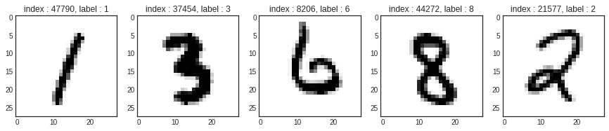
print(f'train_num :{num_x_train}\t val_num : {num_x_val}\t test_num : {num_x_test}')train_num :42000 val_num : 18000 test_num : 10000num_sample = 5
randim_idx = np.random.randint(60000, size=num_sample)
plt.figure(figsize=(15, 3))
for i, idx in enumerate(randim_idx):
img = x_train_full[idx, :]
label = y_train_full[idx]
plt.subplot(1, len(randim_idx), i+1)
plt.imshow(img)
plt.title(f'index : {idx}, label : {label}')
x_train = x_train/255.
x_val = x_val/255.
x_test = x_test/255.

y_train = to_categorical(y_train)
y_val = to_categorical(y_val)
y_test = to_categorical(y_test)
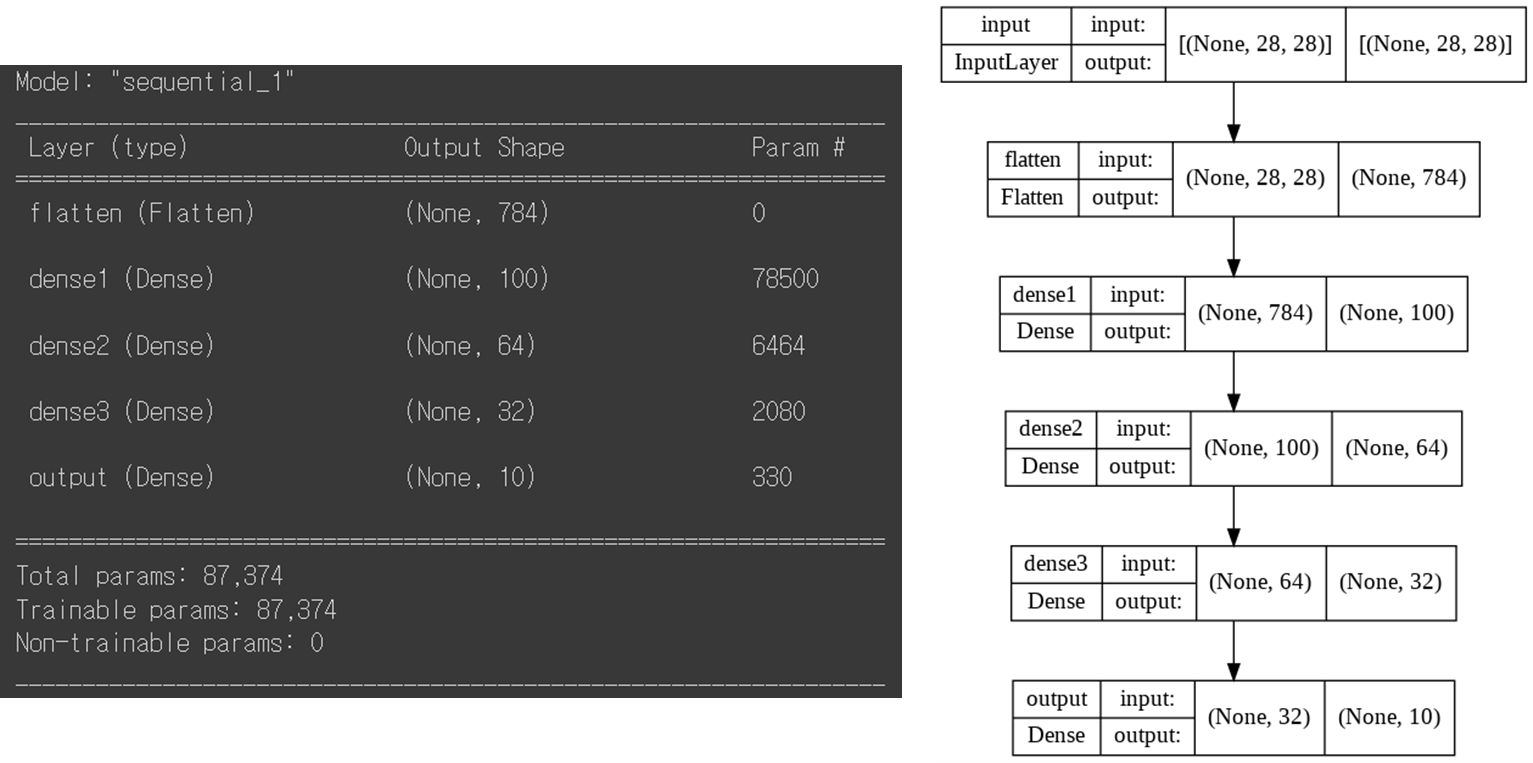
모델구성
model = Sequential([Input(shape=(28,28), name='input'),
                    Flatten(input_shape=[28,28], name='flatten'),
                    Dense(100, activation='relu', name='dense1'),
                    Dense(64, activation='relu', name='dense2'),
                    Dense(32, activation='relu', name='dense3'),
                    Dense(10, activation='softmax', name='output')])

model.summary()

plot_model(model, show_shapes=True)
모델 컴파일 및 학습
model.compile(loss='categorical_crossentropy',
              optimizer='sgd',
              metrics=['accuracy'])
history = model.fit(x_train, y_train,
epochs=50,
batch_size=128,
validation_data=(x_val, y_val))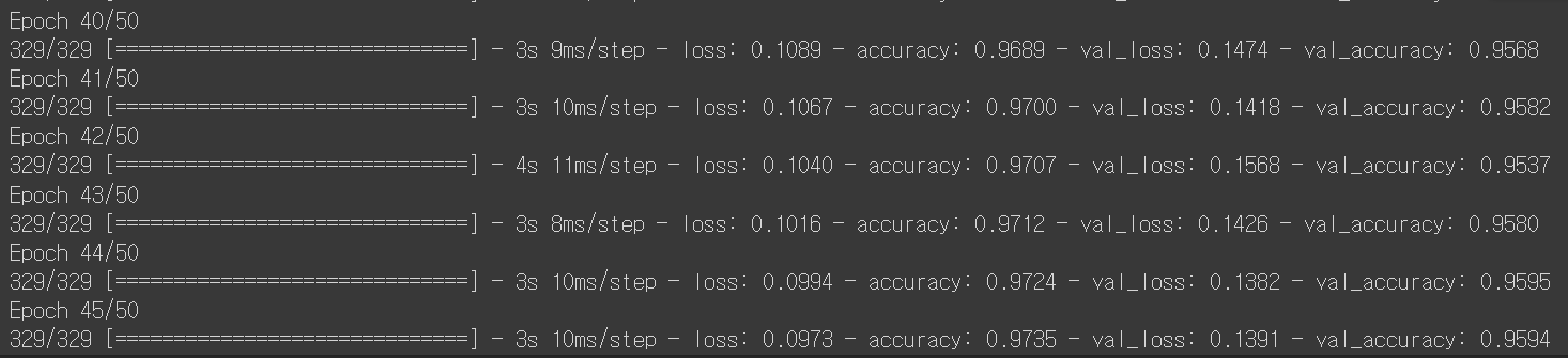
history_dict = history.history
loss = history_dict['loss']
val_loss = history_dict['val_loss']

epochs = range(1, len(loss)+1)
fig = plt.figure(figsize=(12,5))

ax1 = fig.add_subplot(1, 2, 1)
ax1.plot(epochs, loss, color='blue', label='train_loss')
ax1.plot(epochs, val_loss, color='red', label='val_loss')
ax1.set_title('Train and Validation Loss')
ax1.set_xlabel('Epochs')
ax1.set_ylabel('Loss')
ax1.grid()
ax1.legend()

accuracy = history_dict['accuracy']
val_accuracy = history_dict['val_accuracy']

ax2 = fig.add_subplot(1, 2, 2)
ax2.plot(epochs, accuracy, color='blue', label='accuracy')
ax2.plot(epochs, val_accuracy, color='red', label='val_accuracy')
ax2.set_title('Train and Validation Accuracy')
ax2.set_xlabel('Epochs')
ax2.set_ylabel('Accuracy')
ax2.grid()
ax2.legend()

plt.show()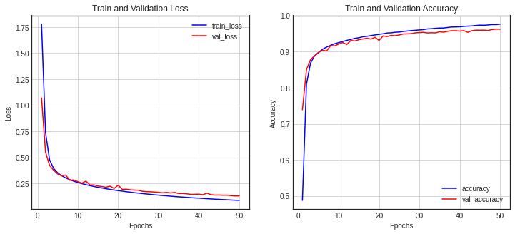
모델 평가 및 예측
model.evaluate(x_test, y_test)
pred_ys = model.predict(x_test)
print(pred_ys.shape)

np.set_printoptions(precision=7)
print(pred_ys[0])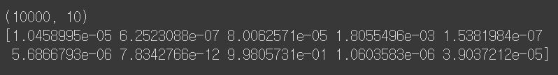
arg_pred_y = np.argmax(pred_ys, axis=1)
plt.imshow(x_test[0])
plt.title(f'pred_label : {arg_pred_y[0]}')
plt.show()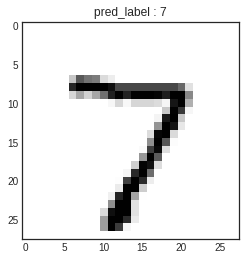
혼동행렬
from sklearn.metrics import classification_report, confusion_matrix
import seaborn as sns
sns.set(style='white')

plt.figure(figsize=(8,8))
cm = confusion_matrix(np.argmax(y_test, axis=1), np.argmax(pred_ys, axis=1))
sns.heatmap(cm, annot=True, fmt='d', cmap='Blues')
plt.xlabel('Predicted Label')
plt.ylabel('True Label')
plt.show()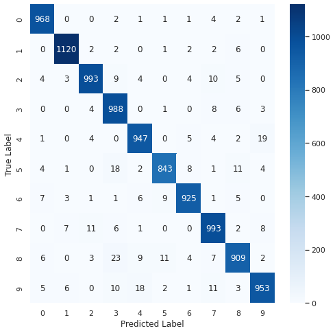
print(classification_report(np.argmax(y_test, axis=1), np.argmax(pred_ys, axis=1)))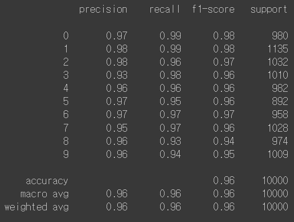
'TF' 카테고리의 다른 글
| [TF] CNN 컨볼루션 신경망 (0) | 2022.04.13 |
|---|---|
| [TF] 딥러닝 학습기술 (0) | 2022.04.12 |
| [TF] 모델의 저장, callbacks (0) | 2022.04.11 |
| [TF] Layer, Model, 모델구성 (0) | 2022.04.11 |