import tensorflow as tf
from tensorflow.keras.datasets.mnist import load_data
from tensorflow.keras.models import Sequential
from tensorflow.keras import models
from tensorflow.keras.layers import Dense, Flatten, Input
from tensorflow.keras.utils import to_categorical, plot_model

from sklearn.model_selection import train_test_split
import numpy as np
import matplotlib.pyplot as plt
plt.style.use('seaborn-white')
- 가장 간단한 방법이라고 할 수 있으며 객체 생성이후 추가하는 방법, 한번에 리스트에 쌓는 방법이 있다
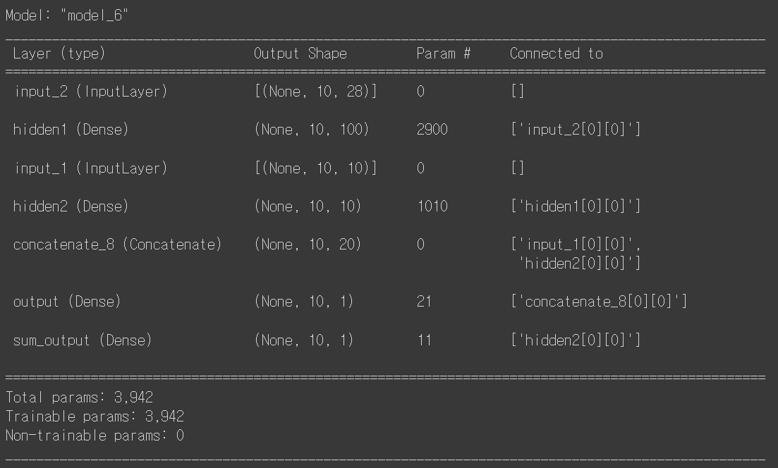
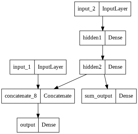
- 다중 입출력이 존재하는 등의 복잡한 모델을 구성할 수 없다.
* 객체에 쌓기
from tensorflow.keras.layers import Dense, Flatten, Activation, Input
from tensorflow.keras.models import Sequential, Model
from tensorflow.keras.utils import plot_model
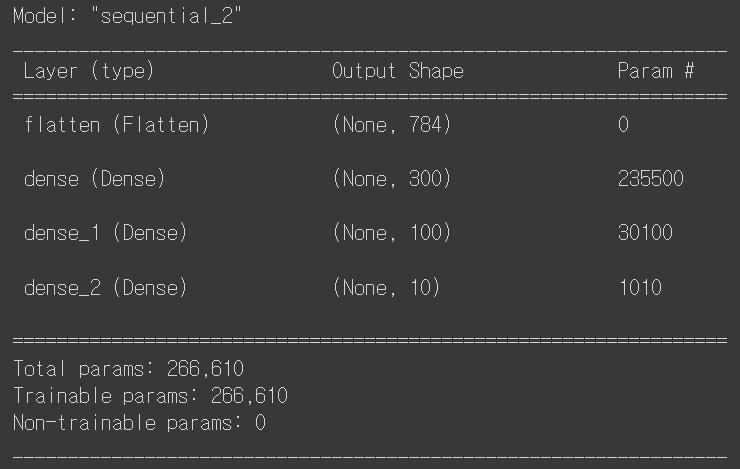
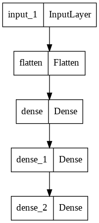
inputs = Input(shape=(28,28,1))
x = Flatten(input_shape=(28,28,1))(inputs)
x = Dense(300, activation='relu')(x)
x = Dense(100, activation='relu')(x)
x = Dense(10, activation='softmax')(x)
model = Model(inputs=inputs, outputs=x)
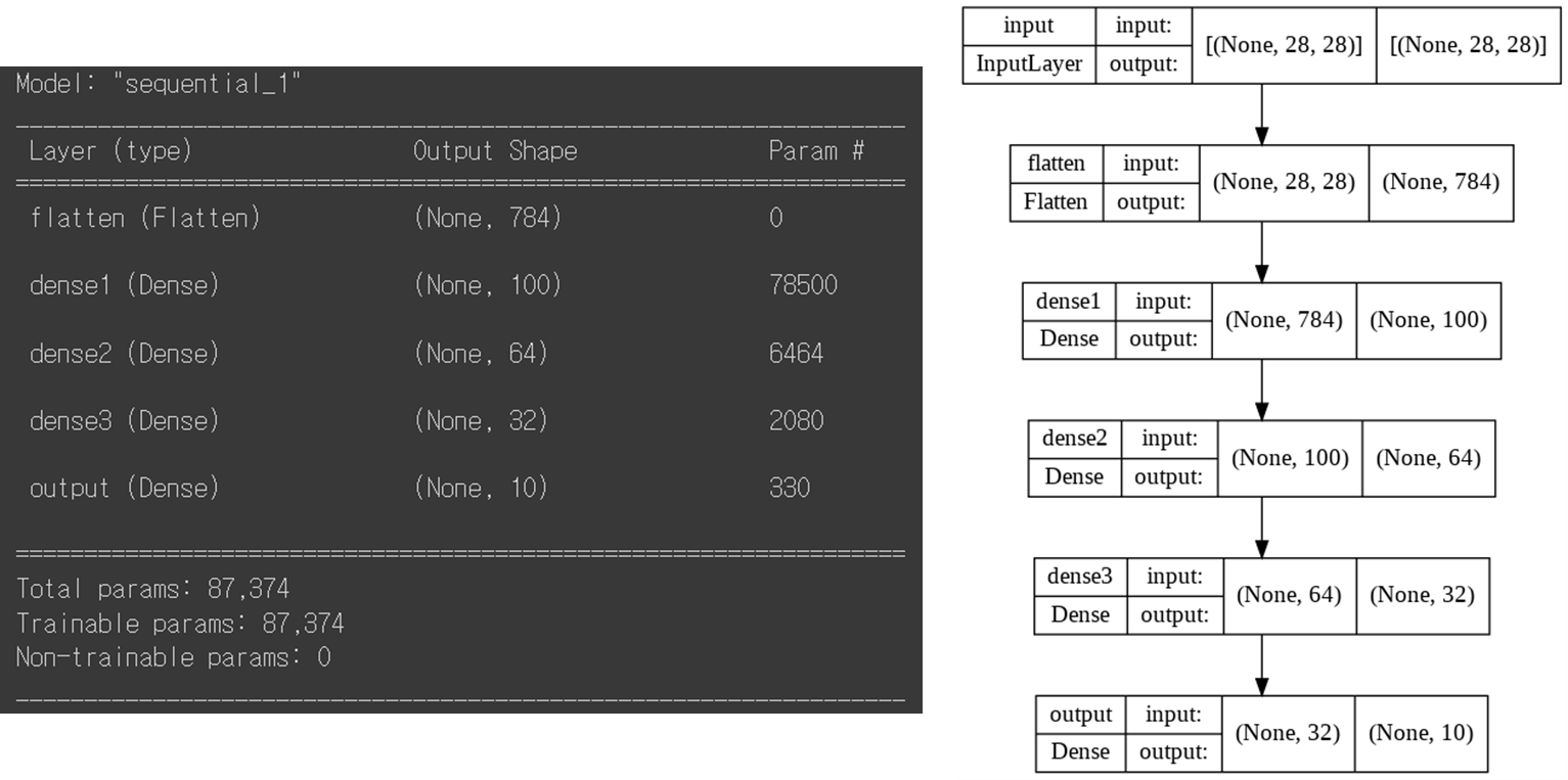
model.summary()
class mymodel(Model):
  def __init__(self, unit=30, activation='relu', **kwargs):
    super(mymodel, self).__init__(**kwargs)
    self.dense_layer1 = Dense(300, activation=activation)
    self.dense_layer2 = Dense(100, activation=activation)
    self.dense_layer3 = Dense(units, activation=activation)
    self.output_layer = Dense(10, activation='softmax')

  def call(self, inputs):
    x = self.dense_layer1(inputs)
    x = self.dense_layer2(x)
    x = self.dense_layer3(x)
    x = self.output_layer(x)
    return x
모델 가중치확인
inputs = Input(shape=(28,28,1))
x = Flatten(input_shape=(28,28,1))(inputs)
x = Dense(300, activation='relu')(x)
x = Dense(100, activation='relu')(x)
x = Dense(10, activation='softmax')(x)

model = Model(inputs=inputs, outputs=x)
model.summary()
model.layers
[<keras.engine.input_layer.InputLayer at 0x7f911aa41090>,
 <keras.layers.core.flatten.Flatten at 0x7f911aa41d90>,
 <keras.layers.core.dense.Dense at 0x7f911a6af950>,
 <keras.layers.core.dense.Dense at 0x7f911a6af590>,
 <keras.layers.core.dense.Dense at 0x7f911aa53590>]